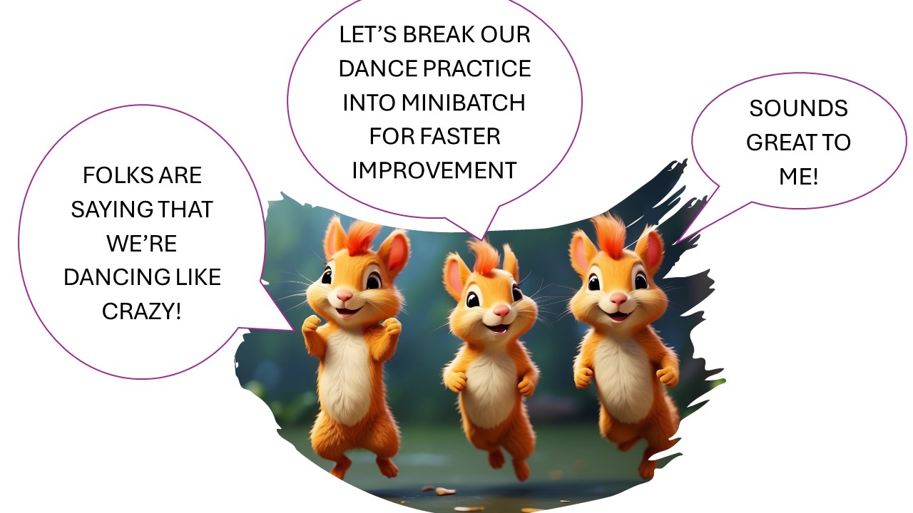
Minibatch learning and variations of Gradient Descent

Minibatch learning in neural networks is akin to dancers learning a complex routine by breaking it down into smaller, manageable sections. This approach allows both the dancers and the neural network to focus on incremental improvement, receiving frequent feedback, and gradually mastering the task through repeated practice.

Just as the routine for dancers is divided into smaller sections to practice each section separately, the training data is divided into smaller subsets of the dataset, i.e., the mini batches.

By dividing, the dancers focus on perfecting one section at a time, the network trains on one minibatch at a time, updating its weights after each minibatch rather than waiting to process the entire dataset. This can lead to faster convergence.

Once all sections are practiced and perfected, the dancers combine them to perform the entire routine, continuously refining their performance. Similarly, after training on all minibatches (completing one epoch), the network has effectively seen the entire dataset. This process is repeated over multiple epochs to further refine the model.

A common batch size in training neural networks is 32 or 64. Batch sizes are often powers of 2 (such as 32 or 64) because computers think in binary, not decimal.

Variants of Gradient Descent

Before continuing, one can review the basics of Gradient Descent. The following are some popular variants of Gradient Descent

Batch Gradient Descent

• Description: Uses the entire dataset to compute the gradient at each step.
• Pros: Converges to the global minimum for convex functions.
• Cons: Computationally expensive for large datasets.

Stochastic Gradient Descent (SGD)

• Description: Stochastic Gradient Descent (SGD) uses one randomly chosen data point (or a few data points) to compute the gradient at each step. This means more updates, i.e., faster. However, it’s like climbing down a mountain, looking only at your steps, not the scene around you. So, the steps can be noisy and may zigzag, not always taking you smoothly downhill.
• Pros: Faster and can escape local minima due to its noisy updates.
• Cons: Noisy updates can cause the loss function to fluctuate.

Mini-batch Gradient Descent

• Description: Uses a small random subset (mini-batch) of the dataset to compute the gradient at each step.
• Pros: Balances the efficiency of batch gradient descent and the robustness of SGD.
• Cons: Requires tuning of the mini-batch size.

Example codes for training with mini-batch in PyTorch

Start by importing necessary modules from PyTorch.

import torch
import torch.nn as nn
import torch.optim as optim
from torch.utils.data import TensorDataset, DataLoader

Create some toy data. Here, x is a tensor of 100 samples, where each sample is a 10-dimensional feature vector, and y is a tensor of 100 target values.

# Toy data
x = torch.randn(100, 10)  # 100 samples, 10 features each
y = torch.randn(100, 1)  # 100 targets

Wrap the data in a Dataset and DataLoader for minibatch training. The DataLoader will allow us to iterate over the dataset in minibatches of size 20.

# Wrap in a Dataset and DataLoader for minibatch training
dataset = TensorDataset(x, y)
data_loader = DataLoader(dataset, batch_size=20)  # Minibatch size of 20

Define a simple model. For this example, we use a feed-forward neural network with a single hidden layer of size 5 and ReLU activation.

# Define a simple model
model = nn.Sequential(
    nn.Linear(10, 5),
    nn.ReLU(),
    nn.Linear(5, 1)
)

Define the loss function as mean squared error, which is a common choice for regression tasks, and an optimizer, in this case, Stochastic Gradient Descent (SGD).

# Define loss function and optimizer
criterion = nn.MSELoss()
optimizer = optim.SGD(model.parameters(), lr=0.01)

Lastly, define the training loop. For each epoch (a full pass over the dataset), iterate over the DataLoader, which yields minibatches of inputs and targets. For each minibatch, perform the forward pass, compute the loss, perform backpropagation to compute gradients, and update the model’s parameters. The loss for the last minibatch of each epoch is printed out.

# Training loop
for epoch in range(50):
    for batch_x, batch_y in data_loader:
        optimizer.zero_grad()
        outputs = model(batch_x)
        loss = criterion(outputs, batch_y)
        loss.backward()
        optimizer.step()

    print(f'Epoch {epoch+1}, Loss: {loss.item()}')

This is a simple example of minibatch training in PyTorch. Most deep learning experiments use this kind of setup where the model is trained on minibatches of data rather than on one sample at a time or on the entire dataset at once.